



LOWFI/1 is the advanced Latent Outlook Weekly Forecasting Interval model. It estimates separate offensive and defensive ratings for every team, in points per game against an average opponent, from scoring trends and a preseason market prior, but is never explicitly told if a team is winning or losing.
This page describes how it works. For why it exists, see the introduction.
Stage 1: Target
A team scoring 30 per game either has a strong offense or has faced weak defenses. The box score does not distinguish them, so the two effects are modeled using a crossed random-effects model fitted across every game since 2004.
The response is points scored in a team-game. Random effects for the scoring offense and the conceding defense, crossed rather than nested, plus a game-level effect. Fixed effects control for home field, week, division games and the league’s scoring environment that season. Fitted via REML.
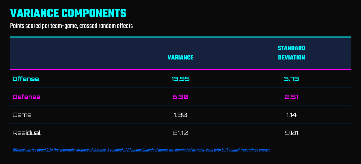
Two important conclusions from the fitting process. Offensive identity has approximately 2.2x the separable variance of defensive identity, so defensive ratings are estimated less precisely across the board. And residual variance of 81 means individual games are noisy, even if both teams’ true ratings are known.
BLUPs are extracted per team-season and centered within season. These are the prediction target: an end-of-season +/- points rating, which is not known during the season.
Stage 2: Preseason prior
LOWFI/1 “seeds” itself for the season with a prior that is built around betting markets and prior season performance.
First, each team’s Vegas win totals and over/under prices are used to construct an implied net rating (i.e. how many points a team is expected to win or lose by against an average team, per game).
This is done by first “de-vigging” the Vegas totals. The totals plus the over/under prices produce implied probabilities, which are then normalized to remove the bookmaker’s margin, and the residual imbalance is converted to a shift in the total:
adj_total = line + sd_wins · Φ⁻¹(p_over)
sd_wins is estimated from the historical dispersion of actual wins around projected totals. A 9.5 at −150/+125 and a 9.5 at +125/−150 are implied to be fairly different teams; the adjustment is worth roughly a third of a win at the extremes.
Once the win totals are adjusted, they are converted to an implied winning percentage (adj_total / games ), which is inverted through a fitted win_pct ~ point_differential relationship to give the expected point differential (i.e. net rating) per game.
This gets close to a preseason prior, but LOWFI/1 tries to estimate offensive and defensive rating separately, so it behooves the model to have the net rating implied by the market split into these priors.
To do so, a ridge regression is used to predict each team’s eventual end-of-season offensive and defensive rating from the market-implied net rating plus their previous season’s offensive, defensive and net ratings. This effectively splits the market into historically accurate offensive and defensive decomposition.
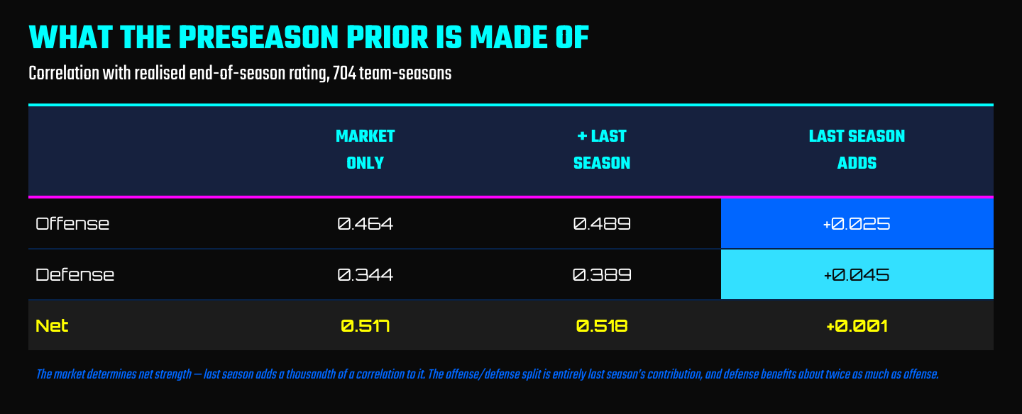
The market determines net strength - prior season information contributes essentially nothing to it. The offense/defense split is entirely the prior season’s contribution.
Net prior correlation with realized strength is 0.518, so the preseason picture accounts for about 27% of variance in end-of-season rating.
Stage 3: In-season estimation
In season “best-guess” true offensive and defensive strengths are estimated using generalized additive models (GAMs), with smoothed terms derived from:
preseason prior (own side and net)
previous season’s ratings (own side and net)
points scored and allowed to date, league-centered
exponentially weighted recent scoring (ρ = 0.9)
opponent quality faced: season-to-date average of opponent ratings, and of opponent preseason priors
tensor interactions of week with the prior, the previous season, and current scoring
In-season terms carry a “has played games” indicator so they contribute nothing before games exist. Observations are weighted so early weeks dominate fitting - equal weighting would give late-season observations (which are near-complete) too much credit and drive a poor fit.
Week 1 uses separate models due to only having priors - fitting a GAM to the full season would lead to pooling across all eighteen weeks, and that would weight the preseason prior by its average usefulness across a season in which in-season scoring carries most of the signal. Measured out of fold, the pooled model was worse at week 1 than the raw prior it was given. The preseason models are therefore fitted only on observations with no games played and uses only four preseason predictors (market estimates and prior season ratings).
Predicted ratings are rescaled per week using coefficients from 5-fold season-blocked cross-validation, correcting systematic over-shrinkage. Post-calibration dispersion ratios run 0.98 at week 1 to 1.00 by week 12.
Standard errors are inflated by a factor decaying in games played - i.e. the ratings should become more certain as more games are accrued. The inflation value is fitted so that simulated win-total dispersion matches the observed dispersion of actual wins around preseason market lines (2.77 against 2.76).
Stage 4: Predicting games
Each game gets an expected spread that is derived from a simple OLS regression on observed home margin of victory using four ratings:
result ~ home_offensive_rating + home_defensive_rating + away_offensive_rating + away_defensive_rating
The intercept of the fitted model is the home field advantage - 2.26 in points. Residual standard error 13.46.
But the spread is not the same thing as the expected distribution of margin of victory - that distribution actually follows from the spread itself, and is not normally distributed around it (for example, margins of victory of +/- 3 or 7 are far more likely than a normal distribution would expect, given the weird point system of football). Instead, an ordered probit over integer margins from −49 to +59 is used to define the distribution, and the spread shifts the location within the distribution
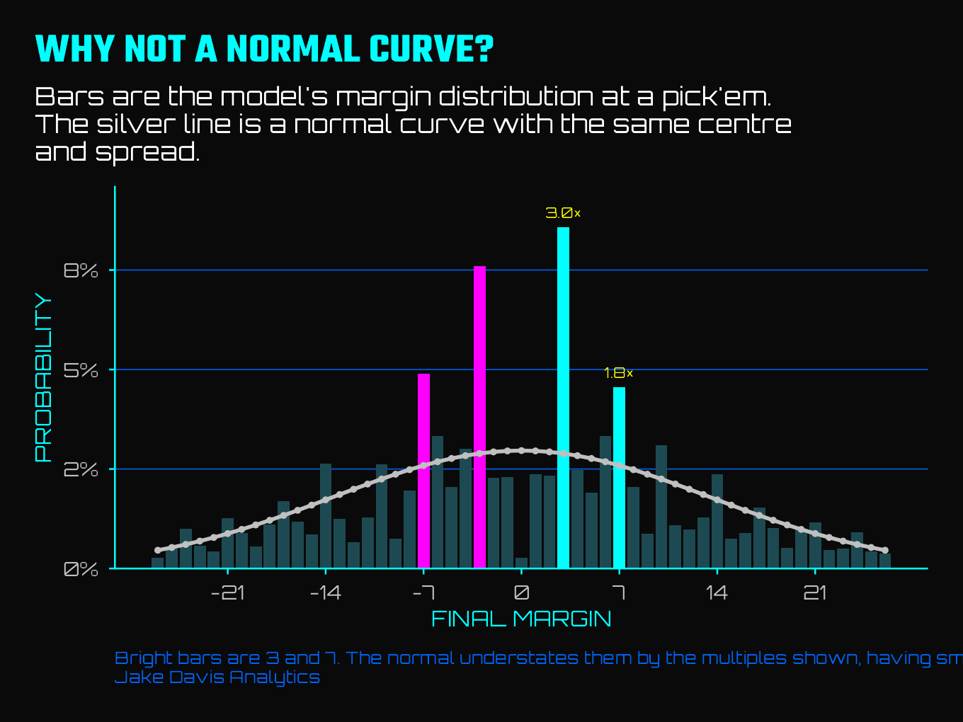
he pmf is precomputed across a grid of spreads and sampled by inverse CDF during simulation to get expected MOV, which is what allows ten thousand seasons to run in seconds.
Stage 5: Simulation
10,000 simulations via nflseedR, with full seeding and tiebreaker rules. Each simulation draws one rating per team from its uncertainty band and holds it for the season, then samples each game from the margin distribution.
Holding the draw is required: redrawing weekly would average out rating uncertainty within each simulated season and understate win-total spread.
Held-out performance
Fitted through 2022, evaluated on 2023–2025 (816 games, unseen):
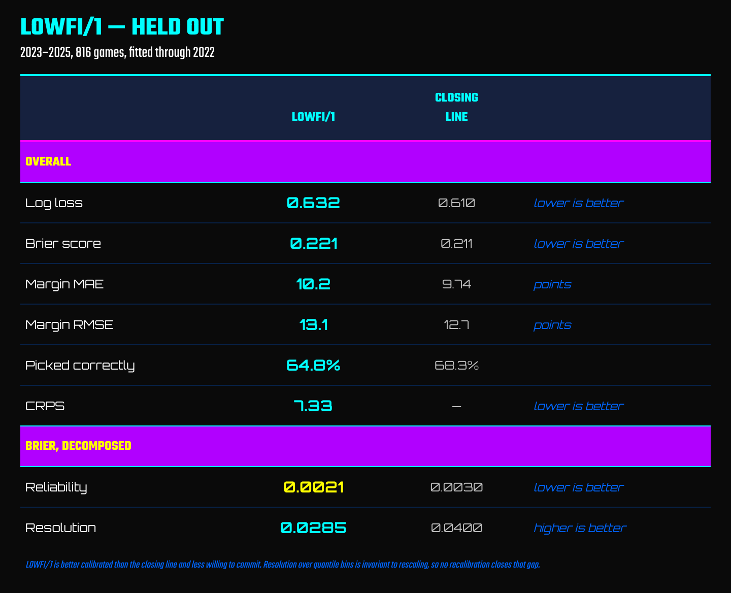
Correlation with the closing line: 0.85. Mean absolute difference: 2.47 points.
LOWFI/1’s reliability is better than the market’s, but resolution is 29% worse. The model is well calibrated, but insufficiently bold.
When examining randomized PIT across held-out games, the result is flat by decile (9.1, 9.7, 10.3, 11.3, 11.4, 10.3, 10.5, 8.5, 8.8, 10.0 against 10 expected), with mean 0.495 and standard deviation 0.282 against 0.289 for a uniform. The margin distributions are well calibrated.
When regressing actual margin on predicted margin out of sample, the slope is 1.02 (se 0.082), consistent with 1 (which is what’s expected for a good margin predictor).
Known limitations
Week 18: Log loss 0.684 against the market’s 0.586. Seeding-driven rest is unobservable from final scores, and so the model struggles to make great predictions.
Preseason compression: Projected win totals are approximately 20% too tightly dispersed at week 0, decaying to 7% by week 8. Costs roughly 1% of accuracy and primarily means there isn’t enough diversity of predicted records early.
Fixed margin shape: The distribution’s location moves with the spread but its scale does not, so equal spreads in high- and low-scoring games receive identical distributions. A location-scale ordered probit conditioning scale on projected total was tested and produced no improvement (CRPS change −0.02%, p = 0.45) because the total model’s R² is 0.053 — the scale covariate is effectively noise.
Neutral sites: International and neutral-site games receive full home field advantage. Approximately eight games per season.
Defensive precision: Defensive ratings are less precisely estimated than offensive ones in every week of every season, following from the variance decomposition in Stage 1.